Great day! I learned how to use vlookup in excel. Here was the problem. I had sent out a cold email to ~2500 podcasters last week. The list of leads I used had a podcaster’s name, email, show id, and show name. Around 40% of people didn’t open the cold email, so I wanted to send a follow-up.

Sendy, the emailing platform, let me download a new list made up of the 40%. But the list only had the lead’s email. I needed the email along with the name, email, show id, and show name to write a cold email people would actually open.

How then would I get a list of the 40% that had all 4 values?

The first thought I had was that I would “subtract” the cold email list from the original email list. I would try and find a formula which would copy a lead from the original list into a new list if it matched with the email from the list of unopened. So I googled around and tried to figure out how to subtract one list from another.

That was unsatisfying because I was looking at the problem backwards!

It turns out that I needed to take values from the original list and add it to the unopened list – specifically name, show id, and show name. And that’s exactly what vlookup lets you do super quickly.

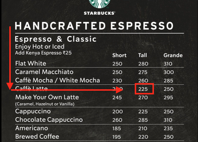
At its most basic, a vlookup does exactly what your eyes did when looking at the photo above. If you wanted to find how many calories a tall Caffe Latte had, first you’d look for “Caffe Latte” in the left hand column, then you’d look in that row until you found the number under “Tall.” 225.

The excel formula is =VLOOKUP(lookup_value,table_array,col_index_num, [range_lookup]).

The lookup_value is basically what you want to look for in the left hand column first. the lookup_value from above was Caffe Latte.

table_array is the grid from which you’re trying to pull your value. For us, it was everything in between Flat White at the top left to 250 at the bottom right.

col_index_num is the column # which your value will be in. Since Tall was the 3rd column, col_index_num would be 3.

Lastly, there’s [range_lookup]. It’s supposed to be something about pulling approximate numbers vs exact, but in most cases, you’re going to want exact, which you denote by writing “FALSE”.

Thus, the vlookup formula we’d used to find the number of calories in a caffe latte is =VLOOKUP(Caffe Latte, Flat White:250, 3, FALSE).

The formula looks unfriendly, but only for a bit. I’m writing this blog because I know I’ll have forgotten how to use the formula in a couple of days, and will need to reference this.

You might see now how I used vlookup to fill in the missing values of my unopened list using the values from my original list. To make a long story short, I did it in 5 seconds.

The biggest lesson I learned from this was that the opportunity for just-in-time learning is something that emerges when you’re wrestling with a problem. To get a problem to grip you, you’ve got to spend a lot of time trying to fix it.

Then, you need to pay attention to how you formulate the problem. What exactly is it that you’re trying to accomplish, and what are the individual steps you think you need to take to do so?

Then, be playful. You can’t assume that the solution you have is the easiest, fastest, or most helpful way to do so. Try and see if you can prove your solution wrong. Try to imagine the multiple different ways of tackling the problem, or the steps.

All of this is how you learn just in time.